Clustering the 2019 NFL Teams
Where does your team stand...
This is the third and final in a series where I take data from the 2019 season and conclude which variables affected NFL franchises the most, as well as other forms of analysis.
Click here for all other articles in the series
The 2020 NFL season is upon us, and despite my reservations about the season starting let alone finishing, now is an appropriate time to group the NFL teams in the 2019 season. For this statistical analysis, I will create a cluster dendrogram using the variables win percentage, point differential, OSRS (Offensive Simple Rating System), and DSRS (Defensive Simple Rating System).
Important Notes:
The main purpose of this article is to group teams based on their similarities in the variables mentioned above. Skip to Model Interpretation if you do not want to read the heavily statistical-oriented sections.
Only regular-season statistics used All data from Pro Football Reference
Defining the Variables
Win percentage
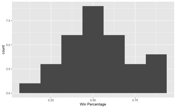
As previously mentioned in my article “Does Strength of Schedule Impact Win Percentage in the NFL?”, win percentage is the proportion, in a decimal format, of games an NFL team won during the 2019 regular-season. The distribution is typically approximately normal, symmetric, and centered around 0.5 as seen in the histogram.
Point Differential
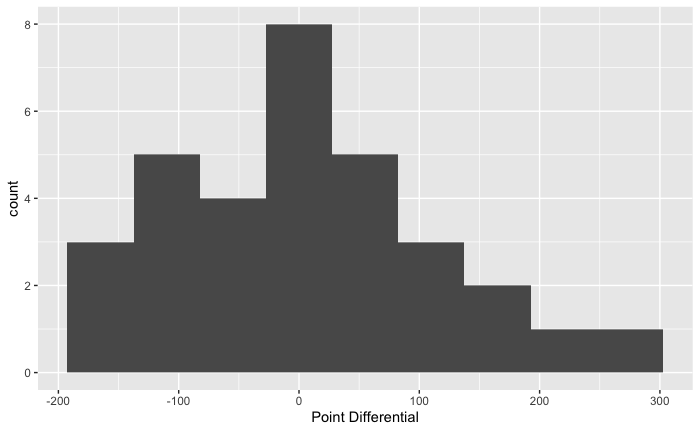
As previously mentioned in my article “Evaluating the Predictability of Win Percentage with Point Differential in the 2019 NFL Season”, point differential is the total sum of the margin of victory or margin of loss throughout an entire season. As expected the center is about zero, and the distribution appears to be approximately normal (or perhaps slightly skewed right).
Point differential was removed in the final model
OSRS
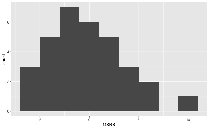
OSRS measures the quality of a team’s offense relative to the average (calculated by Pro Football Reference). Any team above zero is above average and any team below zero is below average. As described by the histogram, the distribution is approximately normal with a potential outlier at 11, the Baltimore Ravens.
DSRS
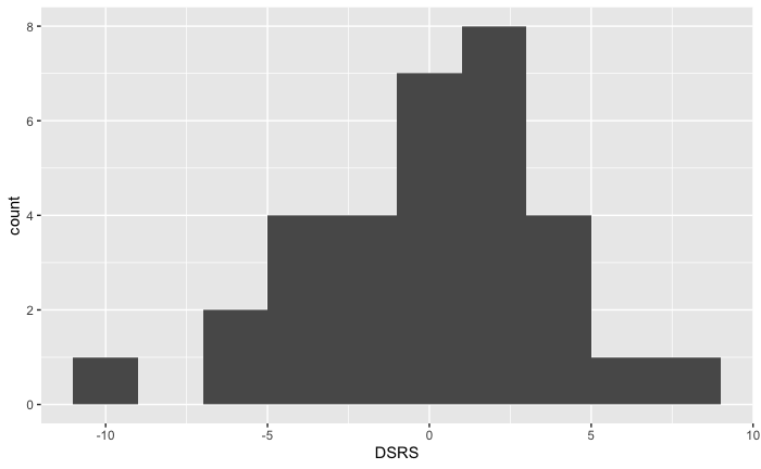
DSRS measures the quality of a team’s defense relative to the average (calculated by Pro Football Reference). Any team above zero is above average and any team below zero is below average. As described by the histogram, the distribution is approximately normal with a potential outlier at -9.1, the Miami Dolphins.
Why these Variables were Chosen or Removed
Win Percentage
Although most including myself would say that there are numerous factors besides a team’s quality that leads to winning, I decided to include it because it loosely does represent the formidability of a team.
OSRS
I included OSRS because I needed to represent both sides of the football and OSRS was how I could incorporate offense
DSRS
I included DSRS in the model because it was a simple way to represent the defensive side of the football.
Point Differential
I removed the point differential because all of the other variables were highly correlated with it. In fact, all of the correlation coefficients were at least 0.8.
Model Creation
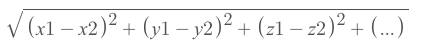
In preparation for a cluster dendrogram, I had to standardize all of the data points for the variables I had selected. Subsequently, I use the Euclidean Distance formula on every data point for each variable for every franchise against all the other franchises.
What is standardization?
Standardization (sometimes known as z-scoring) is taking the individual data point or statistic of a team, subtracting that from the mean and then dividing the difference with the standard deviation.
Example:
Eagles win percentage 2019 = 0.563
Mean win percentage 2019 = 0.500
Standard deviation win percentage 2019 = 0.198
Standardized Score for the Eagles = (0.563 - 0.500)/0.198 = 0.317
Defining the Euclidean Distance Formula
General Formula
Example Formula in Our Model

EaglesW% = Eagles Win Percentage
Repeat this for every possible two team combination. The lower the score the more related the two teams are.
Model Interpretation
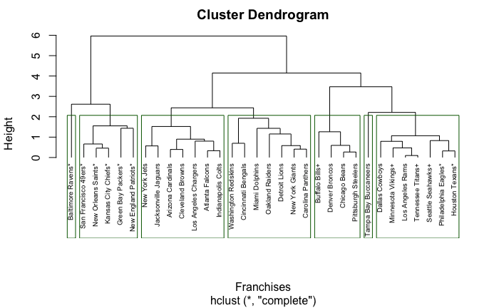
Height is the number of levels in the dendrogram
Complete linkage means that the closer the teams are in the dendrogram the more related they are based on the variables chosen.
Important: The graph is not a team ranking–order does not matter
Naming the Clusters
Cluster One: The Elite Teams
49ers, Saints, Chiefs, Packers, Patriots
These teams were the real championship contenders as seen by the fact that 3 of the final four teams are in this group. These teams were typically above average to elite in all of the statistical categorizes the model incorporated.
However, I would not consider the Packers as a championship contender and if I had included point differential they would not have been in this tier because their differential was 63 compared to the 100+ for the rest of the group.
Cluster Two: Underachievers or Young Teams
Jets, Jaguars, Cardinals, Browns, Chargers, Falcons, Colts
Teams like the Jaguars, Cardinals, and Jets are all teams with young quarterbacks and in many other positions have a young depth-chart. The rest of the teams have top-end talent but were never able to put it together whether it was due to a dysfunctional organization or having their star quarterback retire. However, the fact most of these teams are teams with immense talent that underachieved or young teams is probably a coincidence.
Cluster Three: The Bottom Feeders
Redskins, Bengals, Dolphins, Raiders, Lions, Giants, Panthers
There is not much to say; these were some of the worst teams in the league.
Cluster Four: Defensive Oriented Teams
Bills, Broncos, Bears, Steelers
Most of these teams were vying for a wild-card position and had defensively constructed teams. Three of these teams were in the top five for DSRS.
Cluster Five: Best of Non-Playoff Teams and Worst of the Playoff teams
Cowboys, Vikings, Rams, Titans, Seahawks, Eagles, Texans
All of these teams were border-line playoff teams that could have potentially hosted a Lombardi if the ball bounced their way, but ultimately they were pretenders–not contenders.
Teams’ Without Clusters
Ravens, Buccaneers
Potentially Reasons for No Cluster: Baltimore Ravens
The Ravens 2019 regular season was extremely dominant and as a result, they were essentially elite in every statistic. As previously mentioned, their OSRS was the best in the league at 11 (standardized score of 2.68). Thus, they were not extremely similar to many teams; however, they were somewhat related to cluster one (the contenders).
Potentially Reasons for No Cluster: Tampa Bay Buccaneers
With a quarterback in Jameis Winston that threw for 33 touchdowns, 30 interceptions, and a defense that looked worse than it was in reality because of the turnovers, the Buccaneers were the anomaly of the 2019 NFL season. Thus, they had their own cluster but were loosely similar to the borderline playoff teams.
Side Note: I decided to interpret the model as having five clusters–not the model.
Final Thoughts
The NFL is an ever-changing league, and if I ran this model a year from now the output would probably be completely different. Additionally, if I remade this model again, I would have used a different data set and variables that more specifically represent one aspect of football, for instance, variables that represent special teams.
Follow us on Twitter @flyphillyfly2
All data was via Pro Football Reference
All calculations, models, and graphs were produced using R (Studio).
Featured photo from KeithJJ